Dirty categories: machine learning with non normalized strings

Including strings that represent categories often calls for much data preparation. In particular categories may appear with many morphological variants, when they have been manually input or assembled from diverse sources.

Here we look at a dataset on wages [1] where the column ‘Employee Position Title’ contains dirty categories. On such a column, standard categorical encodings leads to very high dimensions and can lose information on which categories are similar.

We investigate various encodings of this dirty column for the machine learning workflow, predicting the ‘Current Annual Salary’ with gradient boosted trees. First we manually assemble a complex encoder for the full dataframe, after which we show a much simpler way, albeit with less fine control.

[1]

https://www.openml.org/d/42125

The data

We first retrieve the dataset:

from dirty_cat.datasets import fetch_employee_salaries

employee_salaries = fetch_employee_salaries()

X, the input data (descriptions of employees):

X = employee_salaries.X
X

	gender	department	department_name	division	assignment_category	employee_position_title	underfilled_job_title	date_first_hired	year_first_hired
0	F	POL	Department of Police	MSB Information Mgmt and Tech Division Records...	Fulltime-Regular	Office Services Coordinator	NaN	09/22/1986	1986
1	M	POL	Department of Police	ISB Major Crimes Division Fugitive Section	Fulltime-Regular	Master Police Officer	NaN	09/12/1988	1988
2	F	HHS	Department of Health and Human Services	Adult Protective and Case Management Services	Fulltime-Regular	Social Worker IV	NaN	11/19/1989	1989
3	M	COR	Correction and Rehabilitation	PRRS Facility and Security	Fulltime-Regular	Resident Supervisor II	NaN	05/05/2014	2014
4	M	HCA	Department of Housing and Community Affairs	Affordable Housing Programs	Fulltime-Regular	Planning Specialist III	NaN	03/05/2007	2007
...	...	...	...	...	...	...	...	...	...
9223	F	HHS	Department of Health and Human Services	School Based Health Centers	Fulltime-Regular	Community Health Nurse II	NaN	11/03/2015	2015
9224	F	FRS	Fire and Rescue Services	Human Resources Division	Fulltime-Regular	Fire/Rescue Division Chief	NaN	11/28/1988	1988
9225	M	HHS	Department of Health and Human Services	Child and Adolescent Mental Health Clinic Serv...	Parttime-Regular	Medical Doctor IV - Psychiatrist	NaN	04/30/2001	2001
9226	M	CCL	County Council	Council Central Staff	Fulltime-Regular	Manager II	NaN	09/05/2006	2006
9227	M	DLC	Department of Liquor Control	Licensure, Regulation and Education	Fulltime-Regular	Alcohol/Tobacco Enforcement Specialist II	NaN	01/30/2012	2012

9228 rows × 9 columns

and y, our target column (the annual salary):

y = employee_salaries.y
y.name

Out:

'current_annual_salary'

Now, let’s carry out some basic preprocessing:

import pandas as pd

X["date_first_hired"] = pd.to_datetime(X["date_first_hired"])
X["year_first_hired"] = X["date_first_hired"].apply(lambda x: x.year)
# Get a mask of the rows with missing values in 'gender'
mask = X.isna()["gender"]
# And remove them
X.dropna(subset=["gender"], inplace=True)
y = y[~mask]

Assembling a machine-learning pipeline that encodes the data

To build a learning pipeline, we need to assemble encoders for each column, and apply a supervised learning model on top.

The categorical encoders

An encoder is needed to turn a categorical column into a numerical representation:

from sklearn.preprocessing import OneHotEncoder

one_hot = OneHotEncoder(handle_unknown="ignore", sparse=False)

We assemble these to apply them to the relevant columns. The ColumnTransformer is created by specifying a set of transformers alongside with the column names on which each must be applied:

from sklearn.compose import make_column_transformer

encoder = make_column_transformer(
    (one_hot, ["gender", "department_name", "assignment_category"]),
    ("passthrough", ["year_first_hired"]),
    # Last but not least, our dirty column
    (one_hot, ["employee_position_title"]),
    remainder="drop",
)

Pipelining an encoder with a learner

We will use a HistGradientBoostingRegressor, which is a good predictor for data with heterogeneous columns (we need to require the experimental feature for scikit-learn versions earlier than 1.0):

from sklearn.experimental import enable_hist_gradient_boosting

# We can now import the |HGBR| from ensemble
from sklearn.ensemble import HistGradientBoostingRegressor

# We then create a pipeline chaining our encoders to a learner
from sklearn.pipeline import make_pipeline

pipeline = make_pipeline(encoder, HistGradientBoostingRegressor())

Out:

/usr/lib/python3/dist-packages/sklearn/experimental/enable_hist_gradient_boosting.py:16: UserWarning: Since version 1.0, it is not needed to import enable_hist_gradient_boosting anymore. HistGradientBoostingClassifier and HistGradientBoostingRegressor are now stable and can be normally imported from sklearn.ensemble.
  warnings.warn(

The pipeline can be readily applied to the dataframe for prediction:

pipeline.fit(X, y)

Out:

/usr/lib/python3/dist-packages/sklearn/preprocessing/_encoders.py:828: FutureWarning: `sparse` was renamed to `sparse_output` in version 1.2 and will be removed in 1.4. `sparse_output` is ignored unless you leave `sparse` to its default value.
  warnings.warn(
/usr/lib/python3/dist-packages/sklearn/preprocessing/_encoders.py:828: FutureWarning: `sparse` was renamed to `sparse_output` in version 1.2 and will be removed in 1.4. `sparse_output` is ignored unless you leave `sparse` to its default value.
  warnings.warn(

Pipeline(steps=[('columntransformer',
                 ColumnTransformer(transformers=[('onehotencoder-1',
                                                  OneHotEncoder(handle_unknown='ignore',
                                                                sparse=False),
                                                  ['gender', 'department_name',
                                                   'assignment_category']),
                                                 ('passthrough', 'passthrough',
                                                  ['year_first_hired']),
                                                 ('onehotencoder-2',
                                                  OneHotEncoder(handle_unknown='ignore',
                                                                sparse=False),
                                                  ['employee_position_title'])])),
                ('histgradientboostingregressor',
                 HistGradientBoostingRegressor())])

In a Jupyter environment, please rerun this cell to show the HTML representation or trust the notebook.
On GitHub, the HTML representation is unable to render, please try loading this page with nbviewer.org.

Dirty-category encoding

The OneHotEncoder is actually not well suited to the ‘Employee Position Title’ column, as this column contains 400 different entries:

import numpy as np

np.unique(y)

Out:

array([  9196.  ,  11147.24,  13244.5 , ..., 233003.  , 239566.  ,
       303091.  ])

We will now experiment with encoders specially made for handling dirty columns:

from dirty_cat import (
    SimilarityEncoder,
    TargetEncoder,
    MinHashEncoder,
    GapEncoder,
)

encoders = {
    "one-hot": one_hot,
    "similarity": SimilarityEncoder(),
    "target": TargetEncoder(handle_unknown="ignore"),
    "minhash": MinHashEncoder(n_components=100),
    "gap": GapEncoder(n_components=100),
}

We now loop over the different encoding methods, instantiate a new Pipeline each time, fit it and store the returned cross-validation score:

from sklearn.model_selection import cross_val_score

all_scores = dict()

for name, method in encoders.items():
    encoder = make_column_transformer(
        (one_hot, ["gender", "department_name", "assignment_category"]),
        ("passthrough", ["year_first_hired"]),
        # Last but not least, our dirty column
        (method, ["employee_position_title"]),
        remainder="drop",
    )

    pipeline = make_pipeline(encoder, HistGradientBoostingRegressor())
    scores = cross_val_score(pipeline, X, y)
    print(f"{name} encoding")
    print(f"r2 score:  mean: {np.mean(scores):.3f}; std: {np.std(scores):.3f}\n")
    all_scores[name] = scores

Out:

/usr/lib/python3/dist-packages/sklearn/preprocessing/_encoders.py:828: FutureWarning: `sparse` was renamed to `sparse_output` in version 1.2 and will be removed in 1.4. `sparse_output` is ignored unless you leave `sparse` to its default value.
  warnings.warn(
/usr/lib/python3/dist-packages/sklearn/preprocessing/_encoders.py:828: FutureWarning: `sparse` was renamed to `sparse_output` in version 1.2 and will be removed in 1.4. `sparse_output` is ignored unless you leave `sparse` to its default value.
  warnings.warn(
/usr/lib/python3/dist-packages/sklearn/preprocessing/_encoders.py:828: FutureWarning: `sparse` was renamed to `sparse_output` in version 1.2 and will be removed in 1.4. `sparse_output` is ignored unless you leave `sparse` to its default value.
  warnings.warn(
/usr/lib/python3/dist-packages/sklearn/preprocessing/_encoders.py:828: FutureWarning: `sparse` was renamed to `sparse_output` in version 1.2 and will be removed in 1.4. `sparse_output` is ignored unless you leave `sparse` to its default value.
  warnings.warn(
/usr/lib/python3/dist-packages/sklearn/preprocessing/_encoders.py:828: FutureWarning: `sparse` was renamed to `sparse_output` in version 1.2 and will be removed in 1.4. `sparse_output` is ignored unless you leave `sparse` to its default value.
  warnings.warn(
/usr/lib/python3/dist-packages/sklearn/preprocessing/_encoders.py:828: FutureWarning: `sparse` was renamed to `sparse_output` in version 1.2 and will be removed in 1.4. `sparse_output` is ignored unless you leave `sparse` to its default value.
  warnings.warn(
/usr/lib/python3/dist-packages/sklearn/preprocessing/_encoders.py:828: FutureWarning: `sparse` was renamed to `sparse_output` in version 1.2 and will be removed in 1.4. `sparse_output` is ignored unless you leave `sparse` to its default value.
  warnings.warn(
/usr/lib/python3/dist-packages/sklearn/preprocessing/_encoders.py:828: FutureWarning: `sparse` was renamed to `sparse_output` in version 1.2 and will be removed in 1.4. `sparse_output` is ignored unless you leave `sparse` to its default value.
  warnings.warn(
/usr/lib/python3/dist-packages/sklearn/preprocessing/_encoders.py:828: FutureWarning: `sparse` was renamed to `sparse_output` in version 1.2 and will be removed in 1.4. `sparse_output` is ignored unless you leave `sparse` to its default value.
  warnings.warn(
/usr/lib/python3/dist-packages/sklearn/preprocessing/_encoders.py:828: FutureWarning: `sparse` was renamed to `sparse_output` in version 1.2 and will be removed in 1.4. `sparse_output` is ignored unless you leave `sparse` to its default value.
  warnings.warn(
one-hot encoding
r2 score:  mean: 0.776; std: 0.028

/usr/lib/python3/dist-packages/sklearn/preprocessing/_encoders.py:828: FutureWarning: `sparse` was renamed to `sparse_output` in version 1.2 and will be removed in 1.4. `sparse_output` is ignored unless you leave `sparse` to its default value.
  warnings.warn(
/usr/lib/python3/dist-packages/sklearn/preprocessing/_encoders.py:828: FutureWarning: `sparse` was renamed to `sparse_output` in version 1.2 and will be removed in 1.4. `sparse_output` is ignored unless you leave `sparse` to its default value.
  warnings.warn(
/usr/lib/python3/dist-packages/sklearn/preprocessing/_encoders.py:828: FutureWarning: `sparse` was renamed to `sparse_output` in version 1.2 and will be removed in 1.4. `sparse_output` is ignored unless you leave `sparse` to its default value.
  warnings.warn(
/usr/lib/python3/dist-packages/sklearn/preprocessing/_encoders.py:828: FutureWarning: `sparse` was renamed to `sparse_output` in version 1.2 and will be removed in 1.4. `sparse_output` is ignored unless you leave `sparse` to its default value.
  warnings.warn(
/usr/lib/python3/dist-packages/sklearn/preprocessing/_encoders.py:828: FutureWarning: `sparse` was renamed to `sparse_output` in version 1.2 and will be removed in 1.4. `sparse_output` is ignored unless you leave `sparse` to its default value.
  warnings.warn(
similarity encoding
r2 score:  mean: 0.923; std: 0.014

/usr/lib/python3/dist-packages/sklearn/preprocessing/_encoders.py:828: FutureWarning: `sparse` was renamed to `sparse_output` in version 1.2 and will be removed in 1.4. `sparse_output` is ignored unless you leave `sparse` to its default value.
  warnings.warn(
/usr/lib/python3/dist-packages/sklearn/preprocessing/_encoders.py:828: FutureWarning: `sparse` was renamed to `sparse_output` in version 1.2 and will be removed in 1.4. `sparse_output` is ignored unless you leave `sparse` to its default value.
  warnings.warn(
/usr/lib/python3/dist-packages/sklearn/preprocessing/_encoders.py:828: FutureWarning: `sparse` was renamed to `sparse_output` in version 1.2 and will be removed in 1.4. `sparse_output` is ignored unless you leave `sparse` to its default value.
  warnings.warn(
/usr/lib/python3/dist-packages/sklearn/preprocessing/_encoders.py:828: FutureWarning: `sparse` was renamed to `sparse_output` in version 1.2 and will be removed in 1.4. `sparse_output` is ignored unless you leave `sparse` to its default value.
  warnings.warn(
/usr/lib/python3/dist-packages/sklearn/preprocessing/_encoders.py:828: FutureWarning: `sparse` was renamed to `sparse_output` in version 1.2 and will be removed in 1.4. `sparse_output` is ignored unless you leave `sparse` to its default value.
  warnings.warn(
target encoding
r2 score:  mean: 0.842; std: 0.030

/usr/lib/python3/dist-packages/sklearn/preprocessing/_encoders.py:828: FutureWarning: `sparse` was renamed to `sparse_output` in version 1.2 and will be removed in 1.4. `sparse_output` is ignored unless you leave `sparse` to its default value.
  warnings.warn(
/usr/lib/python3/dist-packages/sklearn/preprocessing/_encoders.py:828: FutureWarning: `sparse` was renamed to `sparse_output` in version 1.2 and will be removed in 1.4. `sparse_output` is ignored unless you leave `sparse` to its default value.
  warnings.warn(
/usr/lib/python3/dist-packages/sklearn/preprocessing/_encoders.py:828: FutureWarning: `sparse` was renamed to `sparse_output` in version 1.2 and will be removed in 1.4. `sparse_output` is ignored unless you leave `sparse` to its default value.
  warnings.warn(
/usr/lib/python3/dist-packages/sklearn/preprocessing/_encoders.py:828: FutureWarning: `sparse` was renamed to `sparse_output` in version 1.2 and will be removed in 1.4. `sparse_output` is ignored unless you leave `sparse` to its default value.
  warnings.warn(
/usr/lib/python3/dist-packages/sklearn/preprocessing/_encoders.py:828: FutureWarning: `sparse` was renamed to `sparse_output` in version 1.2 and will be removed in 1.4. `sparse_output` is ignored unless you leave `sparse` to its default value.
  warnings.warn(
minhash encoding
r2 score:  mean: 0.919; std: 0.012

/usr/lib/python3/dist-packages/sklearn/preprocessing/_encoders.py:828: FutureWarning: `sparse` was renamed to `sparse_output` in version 1.2 and will be removed in 1.4. `sparse_output` is ignored unless you leave `sparse` to its default value.
  warnings.warn(
/usr/lib/python3/dist-packages/sklearn/preprocessing/_encoders.py:828: FutureWarning: `sparse` was renamed to `sparse_output` in version 1.2 and will be removed in 1.4. `sparse_output` is ignored unless you leave `sparse` to its default value.
  warnings.warn(
/usr/lib/python3/dist-packages/sklearn/preprocessing/_encoders.py:828: FutureWarning: `sparse` was renamed to `sparse_output` in version 1.2 and will be removed in 1.4. `sparse_output` is ignored unless you leave `sparse` to its default value.
  warnings.warn(
/usr/lib/python3/dist-packages/sklearn/preprocessing/_encoders.py:828: FutureWarning: `sparse` was renamed to `sparse_output` in version 1.2 and will be removed in 1.4. `sparse_output` is ignored unless you leave `sparse` to its default value.
  warnings.warn(
/usr/lib/python3/dist-packages/sklearn/preprocessing/_encoders.py:828: FutureWarning: `sparse` was renamed to `sparse_output` in version 1.2 and will be removed in 1.4. `sparse_output` is ignored unless you leave `sparse` to its default value.
  warnings.warn(
gap encoding
r2 score:  mean: 0.921; std: 0.018

Plotting the results

Finally, we plot the scores on a boxplot:

import seaborn
import matplotlib.pyplot as plt

plt.figure(figsize=(4, 3))
ax = seaborn.boxplot(data=pd.DataFrame(all_scores), orient="h")
plt.ylabel("Encoding", size=20)
plt.xlabel("Prediction accuracy     ", size=20)
plt.yticks(size=20)
plt.tight_layout()

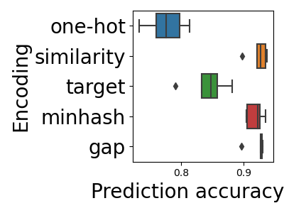
The clear trend is that encoders grasping similarities between categories (SimilarityEncoder, MinHashEncoder, and GapEncoder) perform better than those discarding it.

SimilarityEncoder is the best performer, but it is less scalable on big data than the MinHashEncoder and GapEncoder. The most scalable encoder is the MinHashEncoder. On the other hand, the GapEncoder has the benefit of providing interpretable features (see Investigating and interpreting dirty categories)

A simpler way: automatic vectorization

The code to assemble a column transformer is a bit tedious. We will now explore a simpler, automated, way of encoding the data.

Let’s start again from the raw data:

employee_salaries = fetch_employee_salaries()
X = employee_salaries.X
y = employee_salaries.y

We’ll drop the ‘date_first_hired’ column as it’s redundant with ‘year_first_hired’.

X = X.drop(["date_first_hired"], axis=1)

We still have a complex and heterogeneous dataframe:

X

	gender	department	department_name	division	assignment_category	employee_position_title	underfilled_job_title	year_first_hired
0	F	POL	Department of Police	MSB Information Mgmt and Tech Division Records...	Fulltime-Regular	Office Services Coordinator	NaN	1986
1	M	POL	Department of Police	ISB Major Crimes Division Fugitive Section	Fulltime-Regular	Master Police Officer	NaN	1988
2	F	HHS	Department of Health and Human Services	Adult Protective and Case Management Services	Fulltime-Regular	Social Worker IV	NaN	1989
3	M	COR	Correction and Rehabilitation	PRRS Facility and Security	Fulltime-Regular	Resident Supervisor II	NaN	2014
4	M	HCA	Department of Housing and Community Affairs	Affordable Housing Programs	Fulltime-Regular	Planning Specialist III	NaN	2007
...	...	...	...	...	...	...	...	...
9223	F	HHS	Department of Health and Human Services	School Based Health Centers	Fulltime-Regular	Community Health Nurse II	NaN	2015
9224	F	FRS	Fire and Rescue Services	Human Resources Division	Fulltime-Regular	Fire/Rescue Division Chief	NaN	1988
9225	M	HHS	Department of Health and Human Services	Child and Adolescent Mental Health Clinic Serv...	Parttime-Regular	Medical Doctor IV - Psychiatrist	NaN	2001
9226	M	CCL	County Council	Council Central Staff	Fulltime-Regular	Manager II	NaN	2006
9227	M	DLC	Department of Liquor Control	Licensure, Regulation and Education	Fulltime-Regular	Alcohol/Tobacco Enforcement Specialist II	NaN	2012

9228 rows × 8 columns

The TableVectorizer can to turn this dataframe into a form suited for machine learning.

Using the TableVectorizer in a supervised-learning pipeline

Assembling the TableVectorizer in a Pipeline with a powerful learner, such as gradient boosted trees, gives a machine-learning method that can be readily applied to the dataframe.

The TableVectorizer requires at least dirty_cat 0.2.0.

from dirty_cat import TableVectorizer

pipeline = make_pipeline(
    TableVectorizer(auto_cast=True), HistGradientBoostingRegressor()
)

Let’s perform a cross-validation to see how well this model predicts:

from sklearn.model_selection import cross_val_score

scores = cross_val_score(pipeline, X, y, scoring="r2")

print(f"scores={scores}")
print(f"mean={np.mean(scores)}")
print(f"std={np.std(scores)}")

Out:

scores=[0.91700051 0.90032882 0.93300376 0.93355301 0.93739009]
mean=0.9242552370239272
std=0.013860836102927439

The prediction performed here is pretty much as good as above but the code here is much simpler as it does not involve specifying columns manually.

Analyzing the features created

Let us perform the same workflow, but without the Pipeline, so we can analyze the TableVectorizer’s mechanisms along the way.

table_vec = TableVectorizer(auto_cast=True)

We split the data between train and test, and transform them:

from sklearn.model_selection import train_test_split

X_train, X_test, y_train, y_test = train_test_split(
    X, y, test_size=0.15, random_state=42
)

X_train_enc = table_vec.fit_transform(X_train, y_train)
X_test_enc = table_vec.transform(X_test)

The encoded data, X_train_enc and X_test_enc are numerical arrays:

X_train_enc

Out:

array([[0.00000000e+00, 1.00000000e+00, 0.00000000e+00, ...,
        7.65077591e-02, 7.76393234e-02, 2.00700000e+03],
       [1.00000000e+00, 0.00000000e+00, 0.00000000e+00, ...,
        5.00000000e-02, 5.00000000e-02, 2.00500000e+03],
       [1.00000000e+00, 0.00000000e+00, 0.00000000e+00, ...,
        5.00000000e-02, 5.00000000e-02, 2.00900000e+03],
       ...,
       [1.00000000e+00, 0.00000000e+00, 0.00000000e+00, ...,
        5.00000000e-02, 5.00000000e-02, 1.99000000e+03],
       [0.00000000e+00, 1.00000000e+00, 0.00000000e+00, ...,
        5.00000000e-02, 5.00000000e-02, 2.01200000e+03],
       [1.00000000e+00, 0.00000000e+00, 0.00000000e+00, ...,
        5.00000000e-02, 5.00000000e-02, 2.01400000e+03]])

They have more columns than the original dataframe, but not much more:

X_train.shape, X_train_enc.shape

Out:

((7843, 8), (7843, 169))

Inspecting the features created

The TableVectorizer assigns a transformer for each column. We can inspect this choice:

from pprint import pprint

pprint(table_vec.transformers_)

Out:

[('low_card_cat',
  OneHotEncoder(drop='if_binary', handle_unknown='ignore'),
  ['gender', 'department', 'department_name', 'assignment_category']),
 ('high_card_cat',
  GapEncoder(n_components=30),
  ['division', 'employee_position_title', 'underfilled_job_title']),
 ('remainder', 'passthrough', ['year_first_hired'])]

This is what is being passed to the ColumnTransformer under the hood. If you’re familiar with how the latter works, it should be very intuitive. We can notice it classified the columns ‘gender’ and ‘assignment_category’ as low cardinality string variables. A OneHotEncoder will be applied to these columns.

The vectorizer actually makes the difference between string variables (data type object and string) and categorical variables (data type category).

Next, we can have a look at the encoded feature names.

Before encoding:

X.columns.to_list()

Out:

['gender', 'department', 'department_name', 'division', 'assignment_category', 'employee_position_title', 'underfilled_job_title', 'year_first_hired']

After encoding (we only plot the first 8 feature names):

feature_names = table_vec.get_feature_names_out()
feature_names[:8]

Out:

['gender_F', 'gender_M', 'gender_nan', 'department_BOA', 'department_BOE', 'department_CAT', 'department_CCL', 'department_CEC']

As we can see, it gave us interpretable columns. This is because we used the GapEncoder on the column ‘division’, which was classified as a high cardinality string variable. (default values, see TableVectorizer’s docstring).

In total, we have a reasonable number of encoded columns:

len(feature_names)

Out:

169

Feature importances in the statistical model

In this section, we will train a regressor, and plot the feature importances.

Note:

To minimize computation time, we use the feature importances computed by the RandomForestRegressor, but you should prefer permutation_importance() instead (which are less subject to biases).

First, let’s train the RandomForestRegressor:

from sklearn.ensemble import RandomForestRegressor

regressor = RandomForestRegressor()
regressor.fit(X_train_enc, y_train)

RandomForestRegressor()

In a Jupyter environment, please rerun this cell to show the HTML representation or trust the notebook.
On GitHub, the HTML representation is unable to render, please try loading this page with nbviewer.org.

Retrieving the feature importances:

importances = regressor.feature_importances_
std = np.std([tree.feature_importances_ for tree in regressor.estimators_], axis=0)
indices = np.argsort(importances)
# Sort from least to most
indices = list(reversed(indices))

Plotting the results:

import matplotlib.pyplot as plt

plt.figure(figsize=(12, 9))
plt.title("Feature importances")
n = 20
n_indices = indices[:n]
labels = np.array(feature_names)[n_indices]
plt.barh(range(n), importances[n_indices], color="b", yerr=std[n_indices])
plt.yticks(range(n), labels, size=15)
plt.tight_layout(pad=1)
plt.show()

We can deduce from this data that the three factors that define the most the salary are: being hired for a long time, being a manager, and having a permanent, full-time job :)

The TableVectorizer automates preprocessing

As this notebook demonstrates, many preprocessing steps can be automated by the TableVectorizer, and the resulting pipeline can still be inspected, even with non-normalized entries.