
Note
Click here to download the full example code or to run this example in your browser via Binder
Wikipedia embeddings to enrich the data
When the data comprises common entities (cities, companies or famous people), bringing new information assembled from external sources may be the key to improving the analysis.
Embeddings, or vectorial representations of entities, are a conveniant way to capture and summarize the information on an entity. Relational data embeddings capture all common entities from Wikipedia. [1] These will be called KEN embeddings in the following example.
We will see that these embeddings of common entities significantly improve our results.
The data
We will take a look at the video game sales dataset. Let’s retrieve the dataset:
import pandas as pd

X = pd.read_csv(
    "https://raw.githubusercontent.com/William2064888/vgsales.csv/main/vgsales.csv",
    sep=";",
    on_bad_lines="skip",
)
# Shuffle the data
X = X.sample(frac=1, random_state=11, ignore_index=True)
X.head(3)
Our goal will be to predict the sales amount (y, our target column):
y = X["Global_Sales"]
y
Out:
0        0.26
1        0.05
2        0.02
3        1.16
4        0.03
         ...
16567    0.25
16568    0.49
16569    0.22
16570    0.53
16571    0.11
Name: Global_Sales, Length: 16572, dtype: float64
Let’s take a look at the distribution of our target variable:
import seaborn as sns
import matplotlib.pyplot as plt

sns.set_theme(style="ticks")

sns.histplot(y)
plt.show()
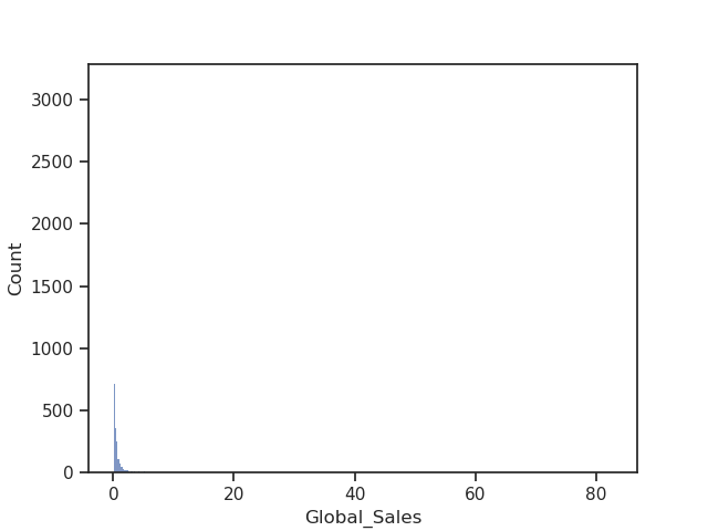
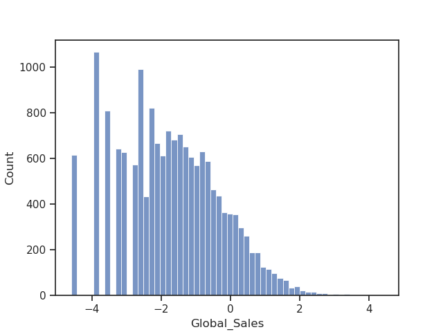
It seems better to take the log of sales rather than the absolute values:
import numpy as np

y = np.log(y)
sns.histplot(y)
plt.show()
Before moving further, let’s carry out some basic preprocessing:
# Get a mask of the rows with missing values in "Publisher" and "Global_Sales"
mask = X.isna()["Publisher"] | X.isna()["Global_Sales"]
# And remove them
X.dropna(subset=["Publisher", "Global_Sales"], inplace=True)
y = y[~mask]
Extracting entity embeddings
We will use KEN embeddings to enrich our data.
We will start by checking out the available tables with
get_ken_table_aliases:
from dirty_cat.datasets import get_ken_table_aliases

get_ken_table_aliases()
Out:
{'movies', 'games', 'companies', 'schools', 'all_entities', 'albums'}
The games table is the most relevant to our case.
Let’s see what kind of types we can find in it with the function
get_ken_types:
from dirty_cat.datasets import get_ken_types

get_ken_types(embedding_table_id="games")
Interesting, we have a broad range of topics!
Next, we’ll use get_ken_embeddings
to extract the embeddings of entities we need:
from dirty_cat.datasets import get_ken_embeddings
KEN Embeddings are classified by types.
The get_ken_embeddings function
allows us to specify the types to be included and/or excluded
so as not to load all Wikipedia entity embeddings in a table.
In a first table, we include all embeddings with the type name “game” and exclude those with type name “companies” or “developer”.
embedding_games = get_ken_embeddings(
    types="game",
    exclude="companies|developer",
    embedding_table_id="games",
)
In a second table, we include all embeddings containing the type name “game_development_companies”, “game_companies” or “game_publish”:
embedding_publisher = get_ken_embeddings(
    types="game_development_companies|game_companies|game_publish",
    embedding_table_id="games",
    suffix="_aux",
)

# We keep the 200 embeddings column names in a list (for the |Pipeline|):
n_dim = 200

emb_columns = [f"X{j}" for j in range(n_dim)]

emb_columns2 = [f"X{j}_aux" for j in range(n_dim)]
Merging the entities
We will now merge the entities from Wikipedia with their equivalent match in our video game sales table:
The entities from the ‘embedding_games’ table will be merged along the column “Name” and the ones from ‘embedding_publisher’ table with the column “Publisher”
from dirty_cat import FeatureAugmenter

fa1 = FeatureAugmenter(tables=[(embedding_games, "Entity")], main_key="Name")
fa2 = FeatureAugmenter(tables=[(embedding_publisher, "Entity")], main_key="Publisher")

X_full = fa1.fit_transform(X)
X_full = fa2.fit_transform(X_full)
Prediction with base features
We will forget for now the KEN Embeddings and build a typical learning pipeline, where will we try to predict the amount of sales only using the base features contained in the initial table.
We first use scikit-learn’s ColumnTransformer to define the columns
that will be included in the learning process and the appropriate encoding of
categorical variables using the MinHashEncoder and OneHotEncoder:
from sklearn.compose import make_column_transformer

from sklearn.preprocessing import OneHotEncoder
from dirty_cat import MinHashEncoder

min_hash = MinHashEncoder(n_components=100)
ohe = OneHotEncoder(handle_unknown="ignore", sparse_output=False)

encoder = make_column_transformer(
    ("passthrough", ["Year"]),
    (ohe, ["Genre"]),
    (min_hash, ["Platform"]),
    remainder="drop",
)
We incorporate our ColumnTransformer into a Pipeline.
We define a predictor, HistGradientBoostingRegressor, fast and reliable for big datasets.
from sklearn.ensemble import HistGradientBoostingRegressor
from sklearn.pipeline import make_pipeline

hgb = HistGradientBoostingRegressor(random_state=0)
pipeline = make_pipeline(encoder, hgb)
The Pipeline can now be readily applied to the dataframe for prediction:
from sklearn.model_selection import cross_validate

# We will save the results in a dictionnary:
all_r2_scores = dict()
all_rmse_scores = dict()

cv_results = cross_validate(
    pipeline, X_full, y, scoring=["r2", "neg_root_mean_squared_error"]
)

all_r2_scores["Base features"] = cv_results["test_r2"]
all_rmse_scores["Base features"] = -cv_results["test_neg_root_mean_squared_error"]

print("With base features:")
print(
    f"Mean R2 is {all_r2_scores['Base features'].mean():.2f} +-"
    f" {all_r2_scores['Base features'].std():.2f} and the RMSE is"
    f" {all_rmse_scores['Base features'].mean():.2f} +-"
    f" {all_rmse_scores['Base features'].std():.2f}"
)
Out:
With base features:
Mean R2 is 0.21 +- 0.01 and the RMSE is 1.30 +- 0.01
Prediction with KEN Embeddings
We will now build a second learning pipeline using only the KEN embeddings from Wikipedia.
We keep only the embeddings columns:
encoder2 = make_column_transformer(
    ("passthrough", emb_columns), ("passthrough", emb_columns2), remainder="drop"
)
We redefine the Pipeline:
pipeline2 = make_pipeline(encoder2, hgb)
Let’s look at the results:
cv_results = cross_validate(
    pipeline2, X_full, y, scoring=["r2", "neg_root_mean_squared_error"]
)

all_r2_scores["KEN features"] = cv_results["test_r2"]
all_rmse_scores["KEN features"] = -cv_results["test_neg_root_mean_squared_error"]

print("With KEN Embeddings:")
print(
    f"Mean R2 is {all_r2_scores['KEN features'].mean():.2f} +-"
    f" {all_r2_scores['KEN features'].std():.2f} and the RMSE is"
    f" {all_rmse_scores['KEN features'].mean():.2f} +-"
    f" {all_rmse_scores['KEN features'].std():.2f}"
)
Out:
With KEN Embeddings:
Mean R2 is 0.37 +- 0.01 and the RMSE is 1.16 +- 0.01
It seems including the embeddings is very relevant for the prediction task at hand!
Prediction with KEN Embeddings and base features
As we have seen the predictions scores in the case when embeddings are only present and when they are missing, we will do a final prediction with all variables included.
We include both the embeddings and the base features:
encoder3 = make_column_transformer(
    ("passthrough", emb_columns),
    ("passthrough", emb_columns2),
    ("passthrough", ["Year"]),
    (ohe, ["Genre"]),
    (min_hash, ["Platform"]),
    remainder="drop",
)
We redefine the Pipeline:
pipeline3 = make_pipeline(encoder3, hgb)
Let’s look at the results:
cv_results = cross_validate(
    pipeline3, X_full, y, scoring=["r2", "neg_root_mean_squared_error"]
)

all_r2_scores["Base + KEN features"] = cv_results["test_r2"]
all_rmse_scores["Base + KEN features"] = -cv_results["test_neg_root_mean_squared_error"]

print("With KEN Embeddings and base features:")
print(
    f"Mean R2 is {all_r2_scores['Base + KEN features'].mean():.2f} +-"
    f" {all_r2_scores['Base + KEN features'].std():.2f} and the RMSE is"
    f" {all_rmse_scores['Base + KEN features'].mean():.2f} +-"
    f" {all_rmse_scores['Base + KEN features'].std():.2f}"
)
Out:
With KEN Embeddings and base features:
Mean R2 is 0.49 +- 0.01 and the RMSE is 1.04 +- 0.01
Plotting the results
Finally, we plot the scores on a boxplot:
plt.figure(figsize=(5, 3))
# sphinx_gallery_thumbnail_number = -1
ax = sns.boxplot(data=pd.DataFrame(all_r2_scores), orient="h")
plt.xlabel("Prediction accuracy     ", size=15)
plt.yticks(size=15)
plt.tight_layout()
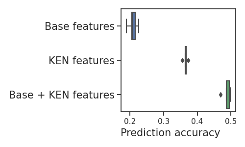
There is a clear improvement when including the KEN embeddings among the explanatory variables.
In this case, the embeddings from Wikipedia introduced additional background information on the game and the publisher of the game that would otherwise be missed.
It helped significantly improve the prediction score.
Total running time of the script: ( 12 minutes 29.308 seconds)