Handling datetime features with the DatetimeEncoder

We illustrate here how to handle datetime features with the DatetimeEncoder.

The DatetimeEncoder breaks down each datetime features into several numerical features, by extracting relevant information from the datetime features, such as the month, the day of the week, the hour of the day, etc. Used in the TableVectorizer, which automatically detects the datetime features, the DatetimeEncoder allows to handle datetime features easily.

import warnings

warnings.filterwarnings("ignore")

Data Importing

We first fetch the dataset.

We want to predict the NO2 air concentration in different cities, based on the date and the time of measurement.

import pandas as pd

data = pd.read_csv(
    "https://raw.githubusercontent.com/pandas-dev/pandas/main/doc/data/air_quality_no2_long.csv"
)
y = data["value"]
X = data[["city", "date.utc"]]
X

	city	date.utc
0	Paris	2019-06-21 00:00:00+00:00
1	Paris	2019-06-20 23:00:00+00:00
2	Paris	2019-06-20 22:00:00+00:00
3	Paris	2019-06-20 21:00:00+00:00
4	Paris	2019-06-20 20:00:00+00:00
...	...	...
2063	London	2019-05-07 06:00:00+00:00
2064	London	2019-05-07 04:00:00+00:00
2065	London	2019-05-07 03:00:00+00:00
2066	London	2019-05-07 02:00:00+00:00
2067	London	2019-05-07 01:00:00+00:00

2068 rows × 2 columns

Encoding the data to numerical representations

Encoders for categorical and datetime features

from sklearn.preprocessing import OneHotEncoder
from dirty_cat import DatetimeEncoder

cat_encoder = OneHotEncoder(handle_unknown="ignore")
# We encode dates using the day of the week as it is probably relevant,
# but no longer than minutes: we are probably not interested in seconds
# and below
datetime_encoder = DatetimeEncoder(add_day_of_the_week=True, extract_until="minute")

from sklearn.compose import make_column_transformer

datetime_columns = ["date.utc"]
categorical_columns = ["city"]

encoder = make_column_transformer(
    (cat_encoder, categorical_columns),
    (datetime_encoder, datetime_columns),
    remainder="drop",
)

Transforming the input data

We can see that the encoder is working as expected: the date feature has been replaced by features for the month, day, hour, and day of the week. Note that the year and minute features have been removed by the encoder because they are constant.

X_ = encoder.fit_transform(X)
encoder.get_feature_names_out()

Out:

array(['onehotencoder__city_Antwerpen', 'onehotencoder__city_London',
       'onehotencoder__city_Paris', 'datetimeencoder__date.utc_month',
       'datetimeencoder__date.utc_day', 'datetimeencoder__date.utc_hour',
       'datetimeencoder__date.utc_dayofweek'], dtype=object)

X_

Out:

array([[ 0.,  0.,  1., ..., 21.,  0.,  4.],
       [ 0.,  0.,  1., ..., 20., 23.,  3.],
       [ 0.,  0.,  1., ..., 20., 22.,  3.],
       ...,
       [ 0.,  1.,  0., ...,  7.,  3.,  1.],
       [ 0.,  1.,  0., ...,  7.,  2.,  1.],
       [ 0.,  1.,  0., ...,  7.,  1.,  1.]])

One-liner with the TableVectorizer

The DatetimeEncoder is used by default in the TableVectorizer, which automatically detects datetime features.

from dirty_cat import TableVectorizer
from pprint import pprint

table_vec = TableVectorizer()
table_vec.fit_transform(X)
pprint(table_vec.get_feature_names_out())

Out:

['date.utc_month',
 'date.utc_day',
 'date.utc_hour',
 'city_Antwerpen',
 'city_London',
 'city_Paris']

If we want the day of the week, we can just replace TableVectorizer’s default parameter:

table_vec = TableVectorizer(
    datetime_transformer=DatetimeEncoder(add_day_of_the_week=True),
)
table_vec.fit_transform(X)
table_vec.get_feature_names_out()

Out:

['date.utc_month', 'date.utc_day', 'date.utc_hour', 'date.utc_dayofweek', 'city_Antwerpen', 'city_London', 'city_Paris']

We can see that the TableVectorizer is indeed using a DatetimeEncoder for the datetime features.

pprint(table_vec.transformers_)

Out:

[('datetime', DatetimeEncoder(add_day_of_the_week=True), ['date.utc']),
 ('low_card_cat',
  OneHotEncoder(drop='if_binary', handle_unknown='ignore'),
  ['city'])]

Predictions with date features

For prediction tasks, we recommend using the TableVectorizer inside a pipeline, combined with a model that uses the features extracted by the DatetimeEncoder.

import numpy as np
from sklearn.ensemble import HistGradientBoostingRegressor
from sklearn.pipeline import make_pipeline

table_vec = TableVectorizer(
    datetime_transformer=DatetimeEncoder(add_day_of_the_week=True),
)
reg = HistGradientBoostingRegressor()
pipeline = make_pipeline(table_vec, reg)

Evaluating the model

When using date and time features, we often care about predicting the future. In this case, we have to be careful when evaluating our model, because standard tools like cross-validation do not respect the time ordering. Instead, we can use the TimeSeriesSplit, which makes sure that the test set is always in the future.

X["date.utc"] = pd.to_datetime(X["date.utc"])
sorted_indices = np.argsort(X["date.utc"])
X = X.iloc[sorted_indices]
y = y.iloc[sorted_indices]

from sklearn.model_selection import TimeSeriesSplit, cross_val_score

cross_val_score(
    pipeline,
    X,
    y,
    scoring="neg_mean_squared_error",
    cv=TimeSeriesSplit(n_splits=5),
)

Out:

array([-120.29551054, -192.65273375, -170.69606296, -225.30467065,
       -214.21981371])

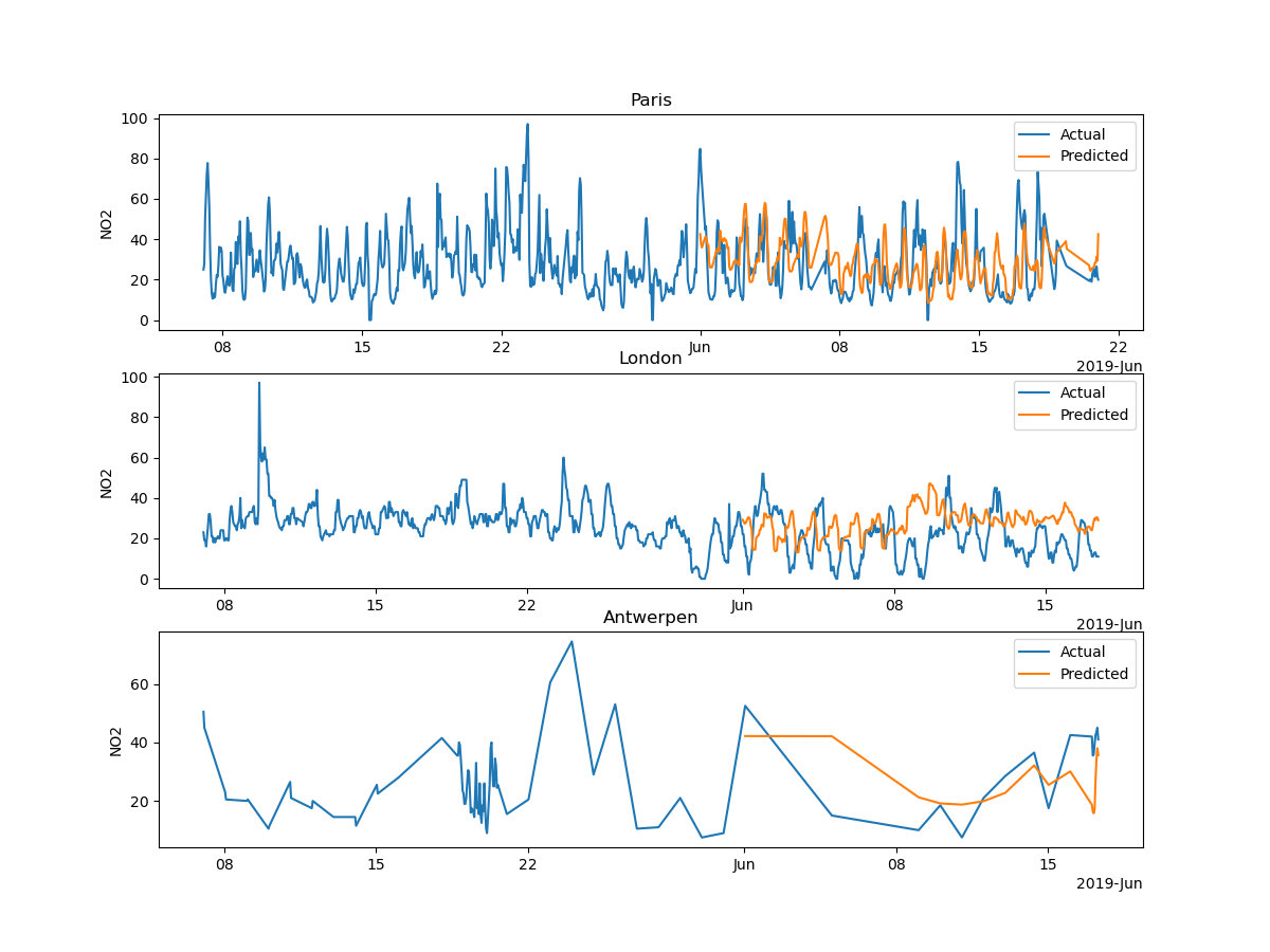
Plotting the prediction

The mean squared error is not obvious to interpret, so we compare visually the prediction of our model with the actual values.

import matplotlib.pyplot as plt
from matplotlib.dates import ConciseDateFormatter

X_train = X[X["date.utc"] < "2019-06-01"]
X_test = X[X["date.utc"] >= "2019-06-01"]

y_train = y[X["date.utc"] < "2019-06-01"]
y_test = y[X["date.utc"] >= "2019-06-01"]

pipeline.fit(X_train, y_train)
fig, axs = plt.subplots(nrows=len(X_test.city.unique()), ncols=1, figsize=(12, 9))

for i, city in enumerate(X_test.city.unique()):
    axs[i].plot(
        X.loc[X.city == city, "date.utc"],
        y.loc[X.city == city],
        label="Actual",
    )
    axs[i].plot(
        X_test.loc[X_test.city == city, "date.utc"],
        pipeline.predict(X_test.loc[X_test.city == city]),
        label="Predicted",
    )
    axs[i].set_title(city)
    axs[i].set_ylabel("NO2")
    axs[i].xaxis.set_major_formatter(
        ConciseDateFormatter(axs[i].xaxis.get_major_locator())
    )
    axs[i].legend()
plt.show()

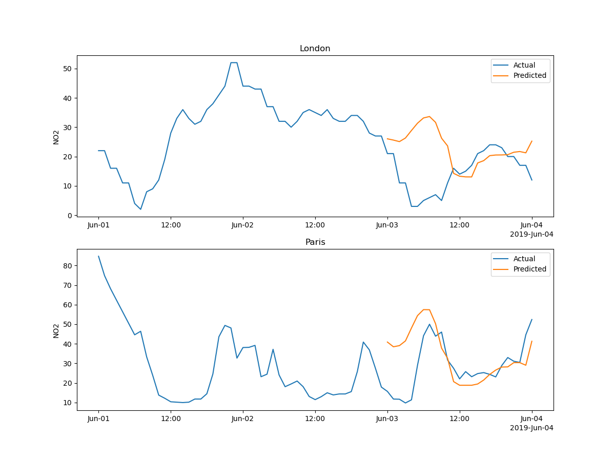
Let’s zoom on a few days:

X_zoomed = X[X["date.utc"] <= "2019-06-04"][X["date.utc"] >= "2019-06-01"]
y_zoomed = y[X["date.utc"] <= "2019-06-04"][X["date.utc"] >= "2019-06-01"]

X_train_zoomed = X_zoomed[X_zoomed["date.utc"] < "2019-06-03"]
X_test_zoomed = X_zoomed[X_zoomed["date.utc"] >= "2019-06-03"]

y_train_zoomed = y[X["date.utc"] < "2019-06-03"]
y_test_zoomed = y[X["date.utc"] >= "2019-06-03"]

pipeline.fit(X_train, y_train)
fig, axs = plt.subplots(
    nrows=len(X_test_zoomed.city.unique()), ncols=1, figsize=(12, 9)
)

for i, city in enumerate(X_test_zoomed.city.unique()):
    axs[i].plot(
        X_zoomed.loc[X_zoomed.city == city, "date.utc"],
        y_zoomed.loc[X_zoomed.city == city],
        label="Actual",
    )
    axs[i].plot(
        X_test_zoomed.loc[X_test_zoomed.city == city, "date.utc"],
        pipeline.predict(X_test_zoomed.loc[X_test_zoomed.city == city]),
        label="Predicted",
    )
    axs[i].set_title(city)
    axs[i].set_ylabel("NO2")
    axs[i].xaxis.set_major_formatter(
        ConciseDateFormatter(axs[i].xaxis.get_major_locator())
    )
    axs[i].legend()
plt.show()

Feature importances

Using the DatetimeEncoder allows us to better understand how the date impacts the NO2 concentration. To this aim, we can compute the importance of the features created by the DatetimeEncoder, using the permutation_importance() function, which basically shuffles a feature and sees how the model changes its prediction.

from sklearn.inspection import permutation_importance

table_vec = TableVectorizer(
    datetime_transformer=DatetimeEncoder(add_day_of_the_week=True),
)

# In this case, we don't use a pipeline, because we want to compute the
# importance of the features created by the DatetimeEncoder
X_ = table_vec.fit_transform(X)
reg = HistGradientBoostingRegressor().fit(X_, y)
result = permutation_importance(reg, X_, y, n_repeats=10, random_state=0)
std = result.importances_std
importances = result.importances_mean
indices = np.argsort(importances)
# Sort from least to most
indices = list(reversed(indices))

plt.figure(figsize=(12, 9))
plt.title("Feature importances")
n = len(indices)
labels = np.array(table_vec.get_feature_names_out())[indices]
plt.barh(range(n), importances[indices], color="b", yerr=std[indices])
plt.yticks(range(n), labels, size=15)
plt.tight_layout(pad=1)
plt.show()

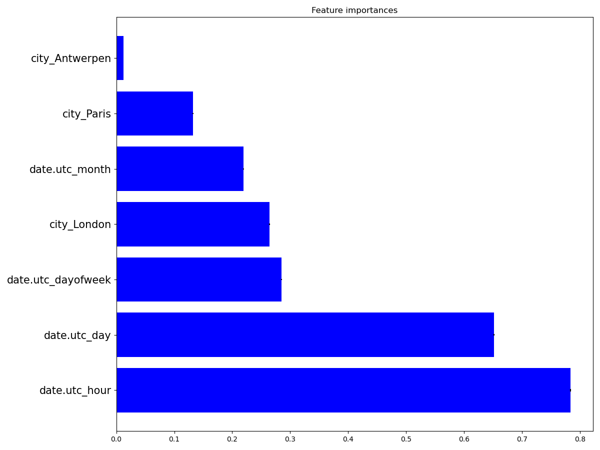
We can see that the hour of the day is the most important feature, which seems reasonable.